Introduction

Organic synthesis plays a vital role in optimizing existing drugs and innovating new drugs. As a significant and challenging research frontier in the field of organic synthesis, cross-coupling reactions have also attracted considerable attention. In the past few years, machine learning has realized great potential in predicting the performance of cross-coupling reactions. However, most of the existing machine learning methods are based on the two-dimensional feature information of the cross-coupling reactions. In order to obtain the coupling reaction features in a multifaceted way, we first explore the three-dimensional and topological descriptors of cross-coupling reactions based on the molecular stick-and-ball model and persistent homology analysis. On this basis, a weighted light convolutional neural network with multi-scale subtraction (OS-MSW) is proposed to extract the deep abstract features of the input descriptors, and the extracted features are applied to LightGBM for yield prediction, thus constructing a highly efficient prediction system, OS-MSWGBM. The experiments demonstrate that OS-MSWGBM exhibits higher efficiency and more accurate prediction results, as well as notably stable prediction performance, which can provide reliable decision-making information for experimental personnel or organizations.

Highlights

• Integrate complex representation (3D geometry & topology) based on the molecular stick-and-ball model and persistent homology analysis.
• Accelerate prediction by constructing an hybrid and efficient yield prediction model.
• Feature descriptor attribution via gradient and eigenmatrix weighting.

Method

1. Topological and 3D Geometric Descriptors

3D Geometric Descriptor

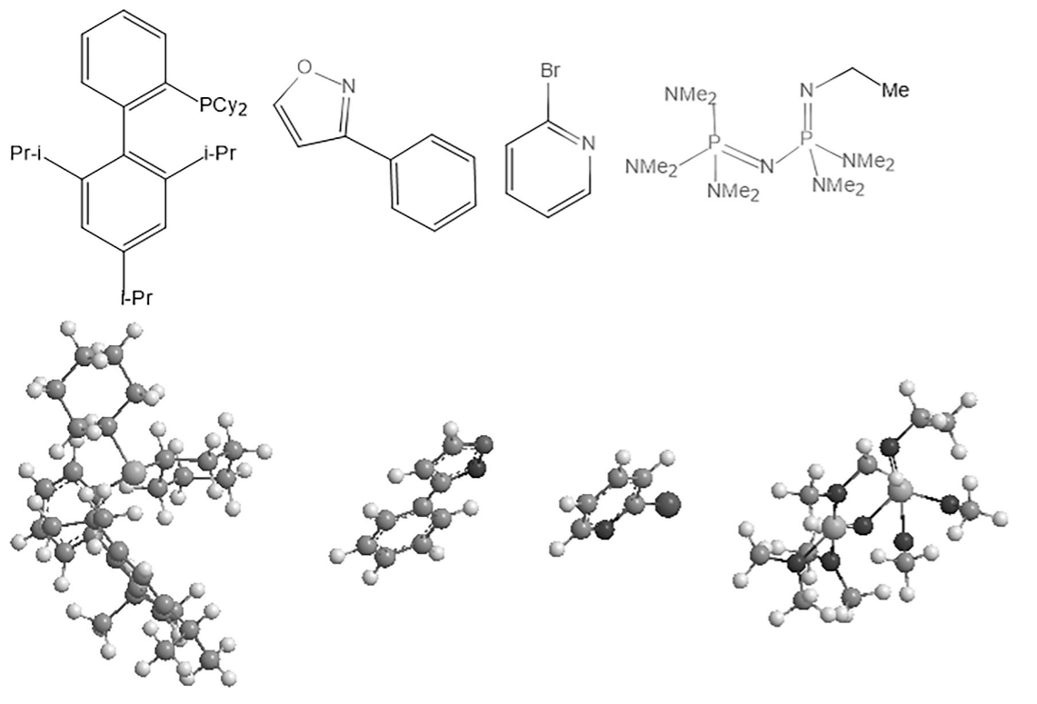
Figure 1. 2D structure formulas and corresponding 3D stick-and-ball models of some reactants.

We compute the spatial and physicochemical descriptors using RDKit and Chem3D, including:

• Molecular Surface Area (MSA) and Molecular Volume (MV) via convex hull algorithms.
• Polar Surface Area (PSA) capturing polar atom contributions.
• Moments of Inertia reflecting mass distribution in 3D.
• Principal Axes Lengths and Radius of Gyration for shape quantification.
• Solvent Accessible Surface Area (SASA) for interaction with solvents.

These descriptors enrich the feature space beyond classical 2D fingerprints, quantify the spatial structural and physicochemical properties of compounds.

Topological Descriptors

We identify and analyze the topological invariants based on persistent homology, such as average lifetimes and persistent entropy of connected components, cycle structures, and void structures.

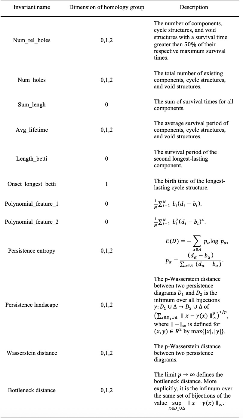
Figure 2. Topological descriptors.

2. Hybrid OS-MSWGBM Network

OS-MSWGBM takes 2D, 3D and topological descriptors as the inputs, learns the deep multi-scale features of them, and finally uses LightGBM to predict yield.

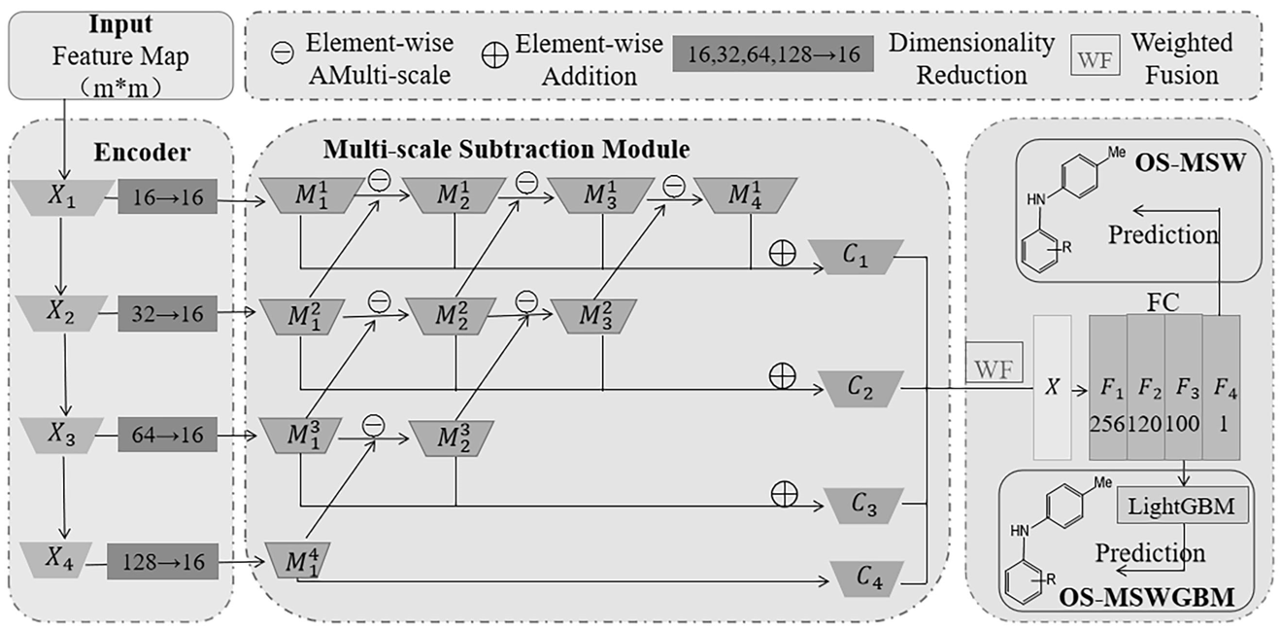
Figure 3. OS-MSWGBM hybrid model.

Multi-Scale Subtraction Weighting (OS-MSW)

• Subtraction Unit. Computes differences between feature maps:

  \[M^{l}_{i+1} = Conv(|M^{l+1}_i - M^{l}_i|),\]

  where \(M^{l}_{i+1}\) captures complementary differences across scales and provides richer information for the decoder.

• Weighted Fusion. Learn weights \(w_i\) via sigmoid-activated pooling:

  \[C_{fused} = \sum_{i=1}^L w_i*C_{i}, \quad w_i = Sigmoid(LinearLayer(\mathrm{pool}(C_{i}))).\]

Combine OS-MSW with LightGBM

• LightGBM Prediction. Optimize the objective function:

  \[\mathcal{L} = \sum_{i} l(y_i, \hat{y}_i) + \Omega(f),\]

  where \(l\) is loss function (e.g., squared error), and \(\Omega\) regularizes tree complexity.

3. Feature Descriptor Attribution

To trace how descriptors contribute to the final prediction, we adopt a gradient weighting technique:

• Gradient Computation. Calculate the gradient \(\nabla_x f\) of the output \(f\) with respect to the input \(x\).

• Weighted Contribution. Multiply the gradient with the input’s feature map block \(A\):

  \[\alpha_i = \sum_{j,k} \nabla_{A_{j,k}} f * A_{i,j,k}\]

  where \(A_{i,j,k}\) is the value of the \(i\)-th channel at location \((j,k)\) in feature map \(A\).

• Normalization. Normalize \(\alpha_i\) to get per-channel weights:

  \[w_i = \frac{\alpha_i}{\sum_i \alpha_i}\]

• Final Attribution. Multiply attribution weights with original inputs to get descriptor-level contribution:

  \[L_{\text{grad-CAM}}(x)_c = \sum_i w_i \cdot x_i\]

Paper | Code | BibTeX